
New Protein Visualizations
distilling insight from complexity; two-dimensional protein–ligand interaction diagrams; protein blob surfaces; space-filling molecule representations

Protein–ligand complexes are great to explore in all their messy glory, but it can be hard to quickly answer basic questions like:
How many hydrogen bonds does this pose form?
Are there any salt bridges stabilizing this interaction?
Does my compound fill the pocket?
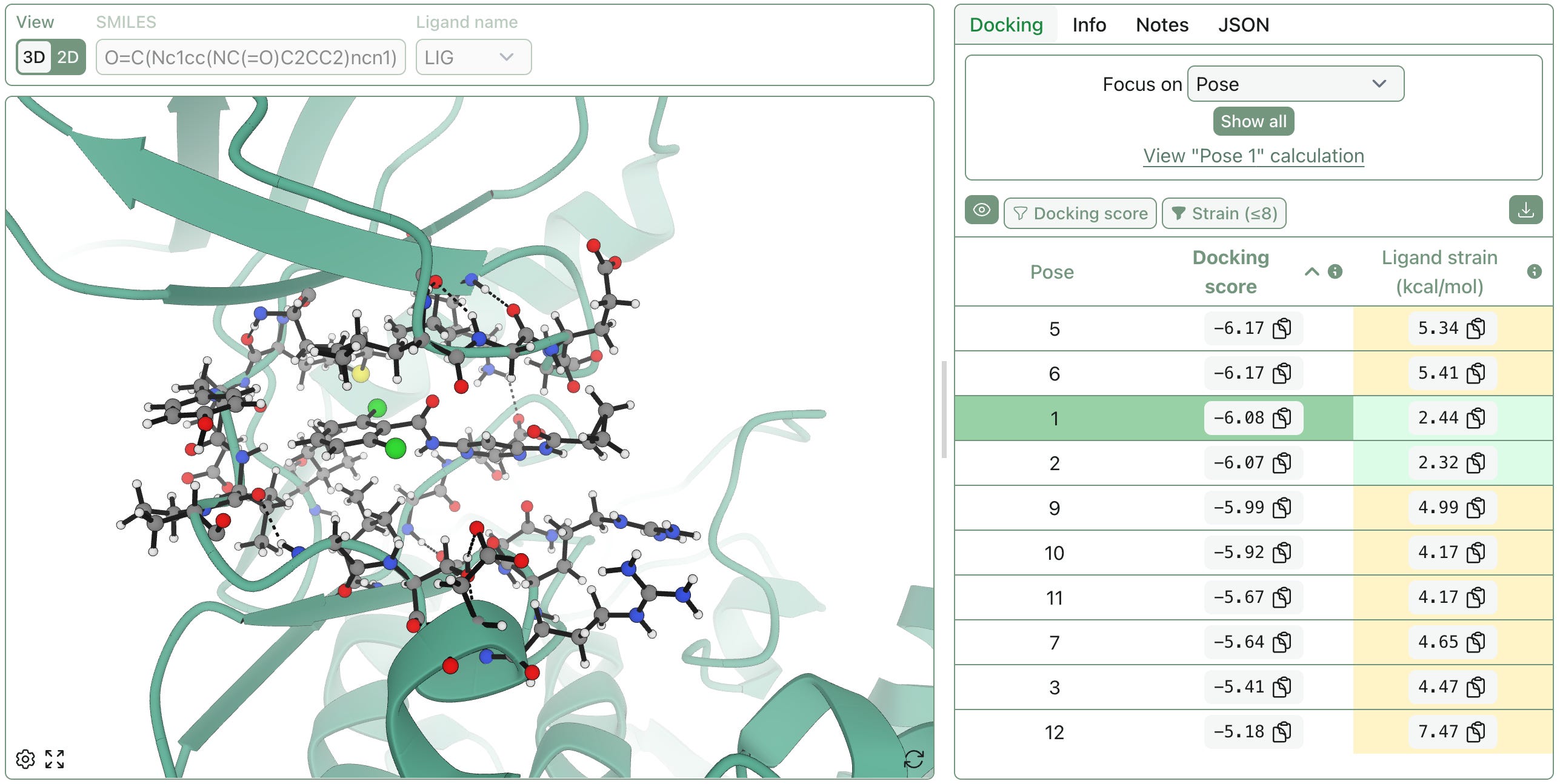
While we’re proud of our default view (below), we’ve been adding new views to make protein–ligand systems easier to interpret and communicate.
Protein–Ligand Interaction Diagrams
No one wants to count hydrogen bonds by squinting at a ribbon diagram during a meeting (or a hackathon). To make key binding-site interactions easier to communicate, we’re introducing a new protein–ligand interaction diagram view:
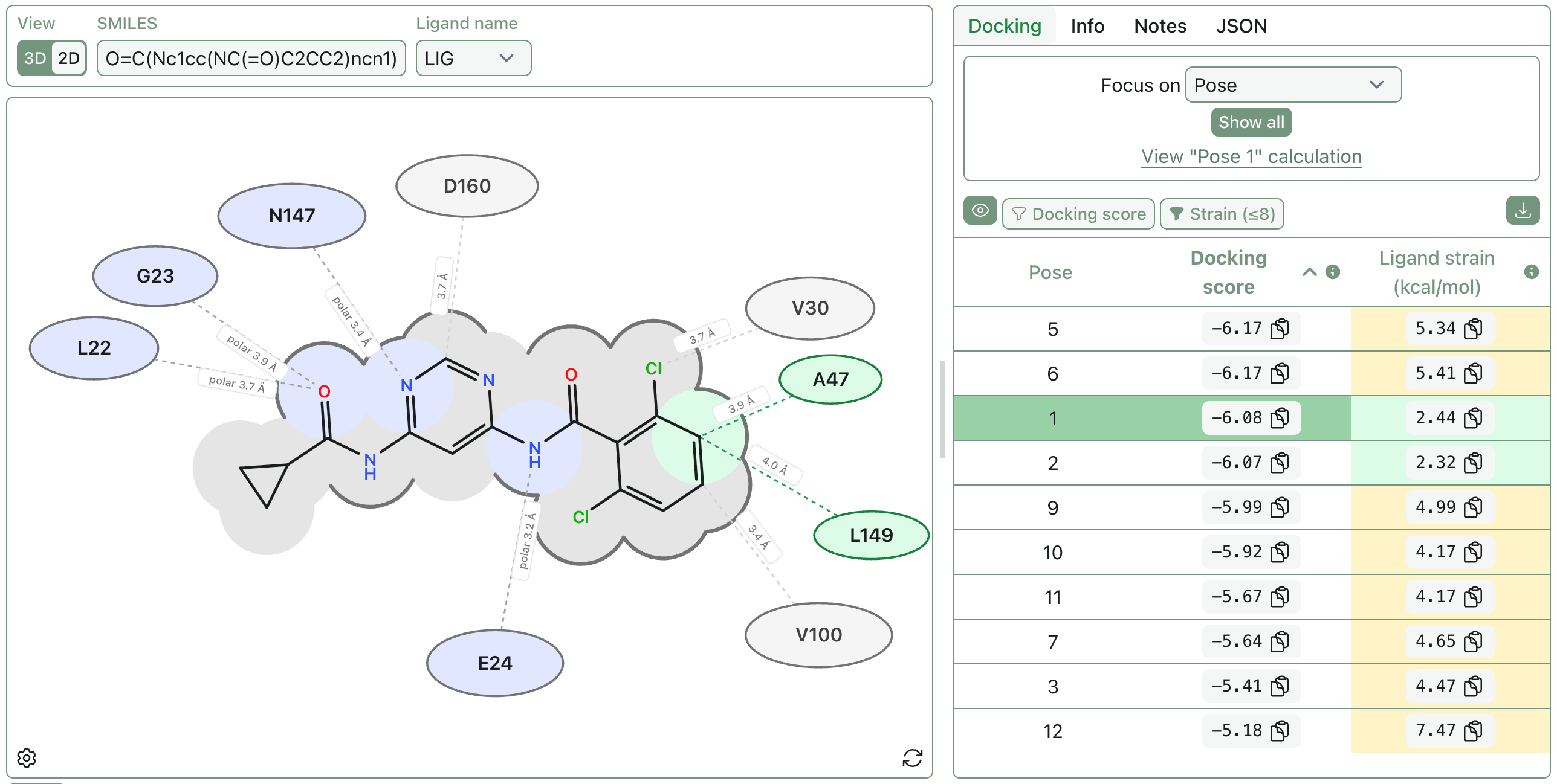
This diagram treats the selected ligand as the center of the binding site, then identifies nearby protein residues and classifies their interactions with the ligand.
If you provide a SMILES string, RDKit is used to draw the ligand; otherwise the ligand layout is inferred from the PDB coordinates. This diagram requires explicit hydrogens, since hydrogen-bond detection depends on donor hydrogen positions.
Hydrogen bonds require a donor–hydrogen–acceptor angle of 120–180°, a donor–acceptor distance of at most 3.5 Å, and a hydrogen–acceptor distance of at most 2.7 Å.
Polar contacts are defined as close contacts between polar heavy atoms (N, O, or S) that are not classified as hydrogen bonds.
Salt bridges are detected between charged ligand atoms and nearby charged residues.
Hydrophobic contacts are close contacts between neutral carbon-like ligand atoms (C or S) and hydrophobic side-chain atoms.
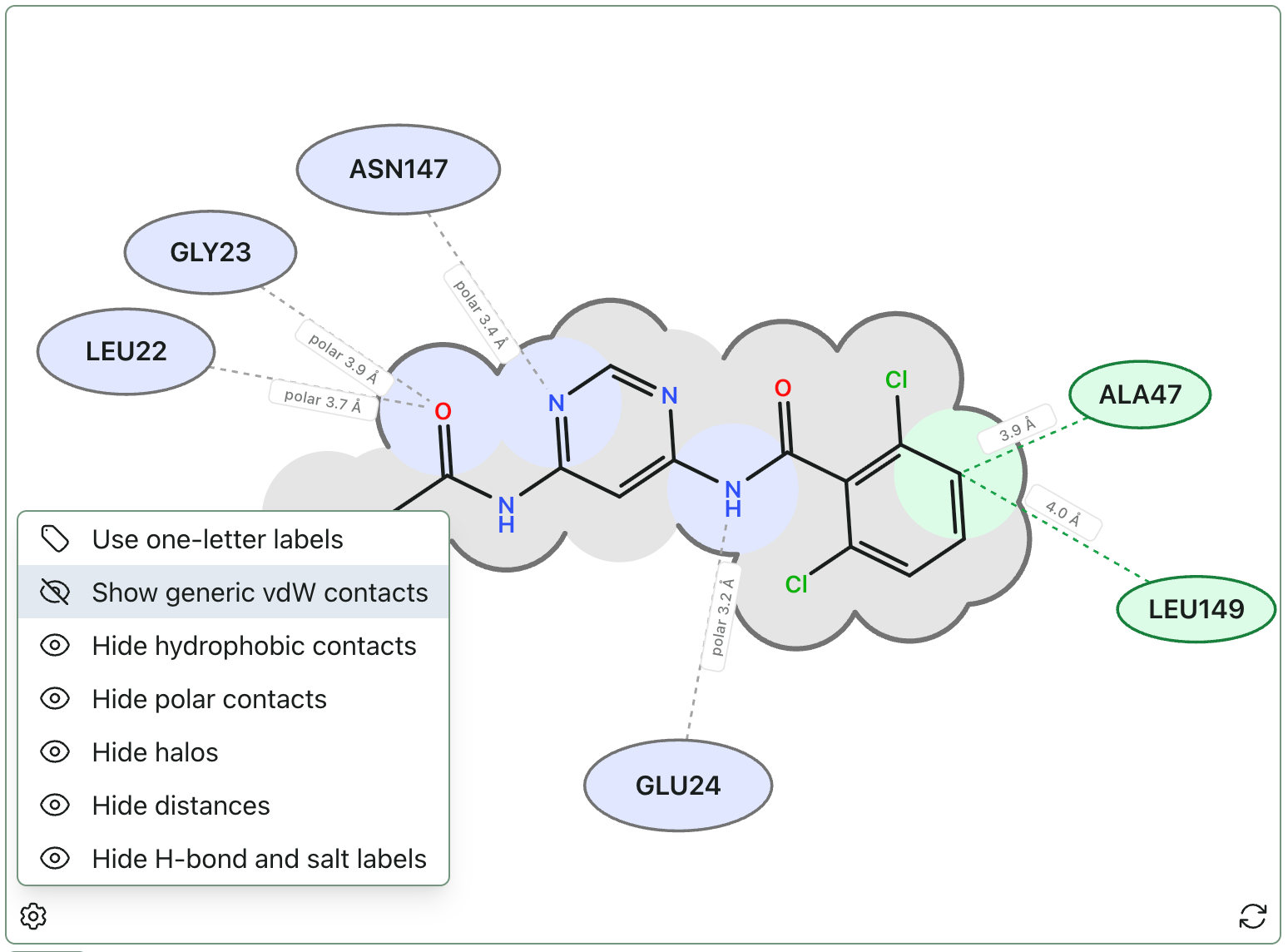
Generic van der Waals contacts are shown with gray residue labels: close heavy-atom contacts that are not classified as hydrogen bonds, salt bridges, polar contacts, or hydrophobic contacts.
Ligand surface outlines help show which parts of the ligand are protein-facing versus solvent-exposed. They are calculated from all the contacts above plus additional nearby residues within 5 Å (up to 100 residues).
This view—like our other views—updates as you switch between poses. The residue labels can be rearranged by clicking and dragging, and the view can be customized further using the settings menu (accessible via the gear icon).
Want to visualize your existing structure? Bring your own file and just use the view: https://labs.rowansci.com/interaction-diagram.
Protein Blob Surface
Another view we’ve received a lot of requests for is a “blob” protein surface view with electrostatic coloring. Different tools generate these surfaces differently, but the general idea is to represent the protein’s volume while highlighting electrostatic character. This makes it a bit more obvious to see how a ligand sits within a pocket, and can be useful for brainstorming e.g. directions where additional atoms could be added.
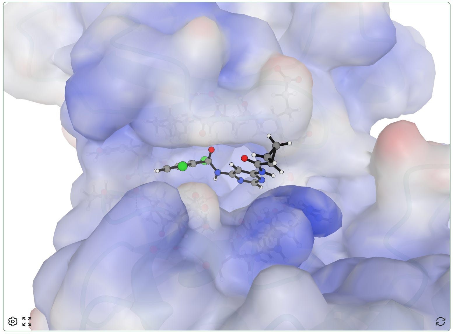
Positive electrostatic potential is shown in blue, while negative electrostatic potential is shown in red.
To make the creation of these views tractable in the browser, we use some heuristics. Atom charges come from the structure when available; otherwise we estimate them from residue and atom names. Similarly, the surface generated is a vdW-like Gaussian surface, not a true solvent-excluded surface.
This view can be accessed via the gear icon in the protein viewer.
Space-Filling Molecules
We’ve also received requests for a space-filling mode for visualizing molecular structures!
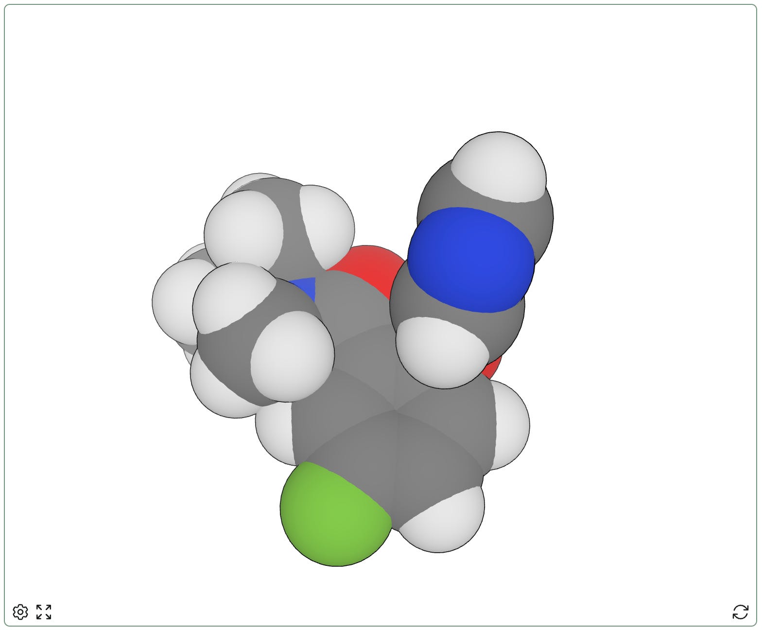
This view can be accessed via the gear icon in the molecule viewer.
If there are views that would be helpful for your research and communications, please let us know at contact@rowansci.com! While we think simulations are cool and fun, clean visualizations matter too. We want Rowan to help bridge the gap between powerful modeling methods and their real-world scientific impact.